Aerodynamics

Aerodynamic Loads

To help with the configuration selection process, an aerodynamic analysis was conducted beforehand to extrapolate the pressure field at the marginal flight conditions. The whole process of calculating pressure coefficients was done in XFLR5, a computational tool for airfoils, wings, and planes.

An important thing to notice about XFLR5 is it uses inviscid theories (LLT, VLM1, VLM2, 3D Panel) which cannot accurately capture pressure gradients at higher Reynolds numbers (>1e7). As the "never exceed" velocity for the reference aircraft equals 230 kts, compressibility effects are expected. Per the note from XFLR5 documentation:

"The VLM and 3D method merely interpolate 2D viscous drag from local wing lift – not great…"

Consequences of this estimation are:

1. Underestimation of total drag
2. Over-estimation of glide ratio and other performance factors

Beyond these limitations, there are more to XFLR5, but these have the greatest impact on the results. As a result of the drawbacks listed above, resultant lift values are greater than those in real life scenarios. These greater lift values then consequently lead to greater loads on the wings, making the wing overbuilt by adding unnecessary mass with added structural elements and additional plies in composite layups.

Because Edge 540 uses a John Roncz symmetrical airfoil which isn't in the public domain so as an alternative NACA0012 airfoil was choosen as the most suitable replacement.

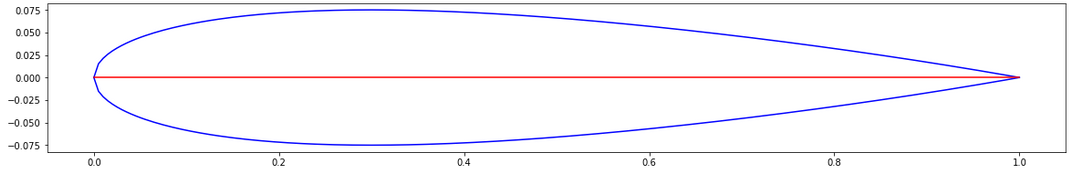
NACA0012 Airfoil

Measurements for the Edge 540 wing were taken out of the Pilot's Operating Handbook and are as follows:

• Wing span – 7.62 m
• Root chord length – 1.68 m
• Tip chord length – 0.84 m

Wings are installed at the mid level and exhibit no dihedral or twist angle.

Airfoil simulations were run for Re < 1×10⁷, after which half-wing runs were conducted. Plane analyses were set to run for angles of attack ranging from -15° to +15° in 1° increments. However, due to the limitations mentioned earlier, the solver could not converge beyond 9.5°.

As a result, the extrapolated pressure field corresponds to flight conditions of 230 kts and an angle of attack of 9°.

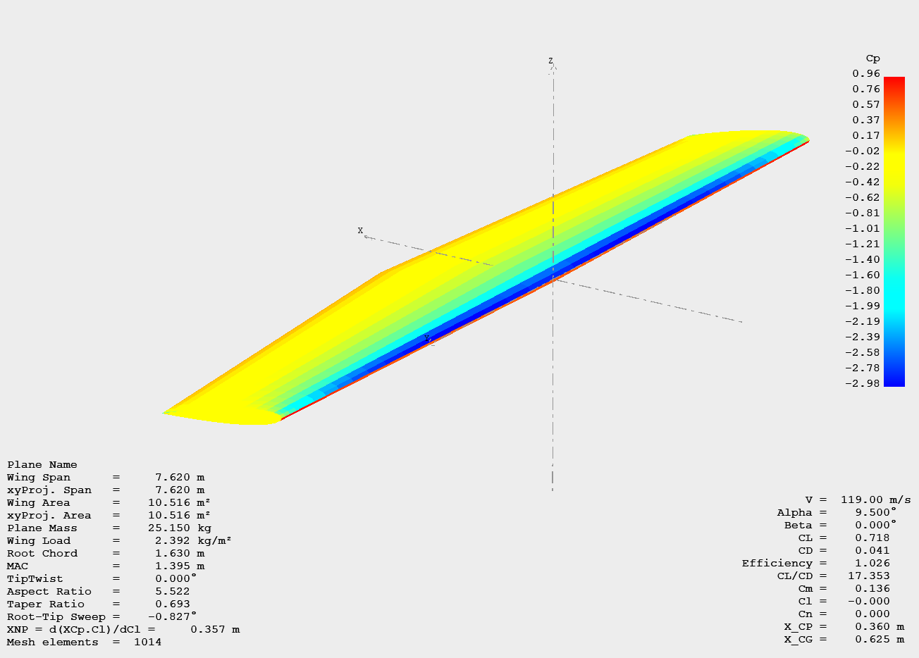
Pressure field on the upper surface of the wing

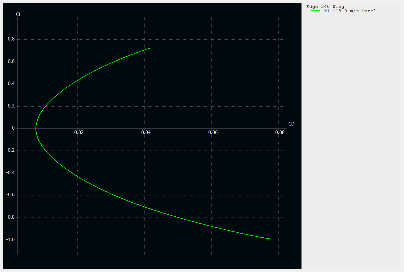
CL/CD plot obtained through 3D Panel method

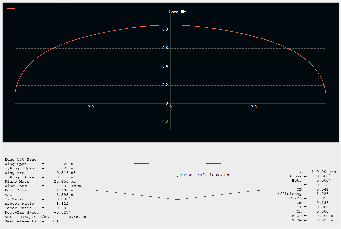
Lift distribution over the wingspan

To get the two-dimensional pressure field, extrapolation of C_p(x) and L(b) curve coordinates was needed (pressure coefficients on upper and lower surfaces were subtracted). These two coordinate sets were then multiplied and normalized to obtain the 2D pressure field.

This field can then be scaled by the loading scalar ½ n m g, where:

• n – loading factor
• m – mass of the airplane
• g – gravitational constant

In this case, the loading scalar equals 0.5 × 726 × 9.81 × 12 = 42732.36 N. 1/2 in this case just means half of the mass since the calculations were done for one wing only.

All of the calculations were done in MATLAB. The resultant pressure field is presented below.

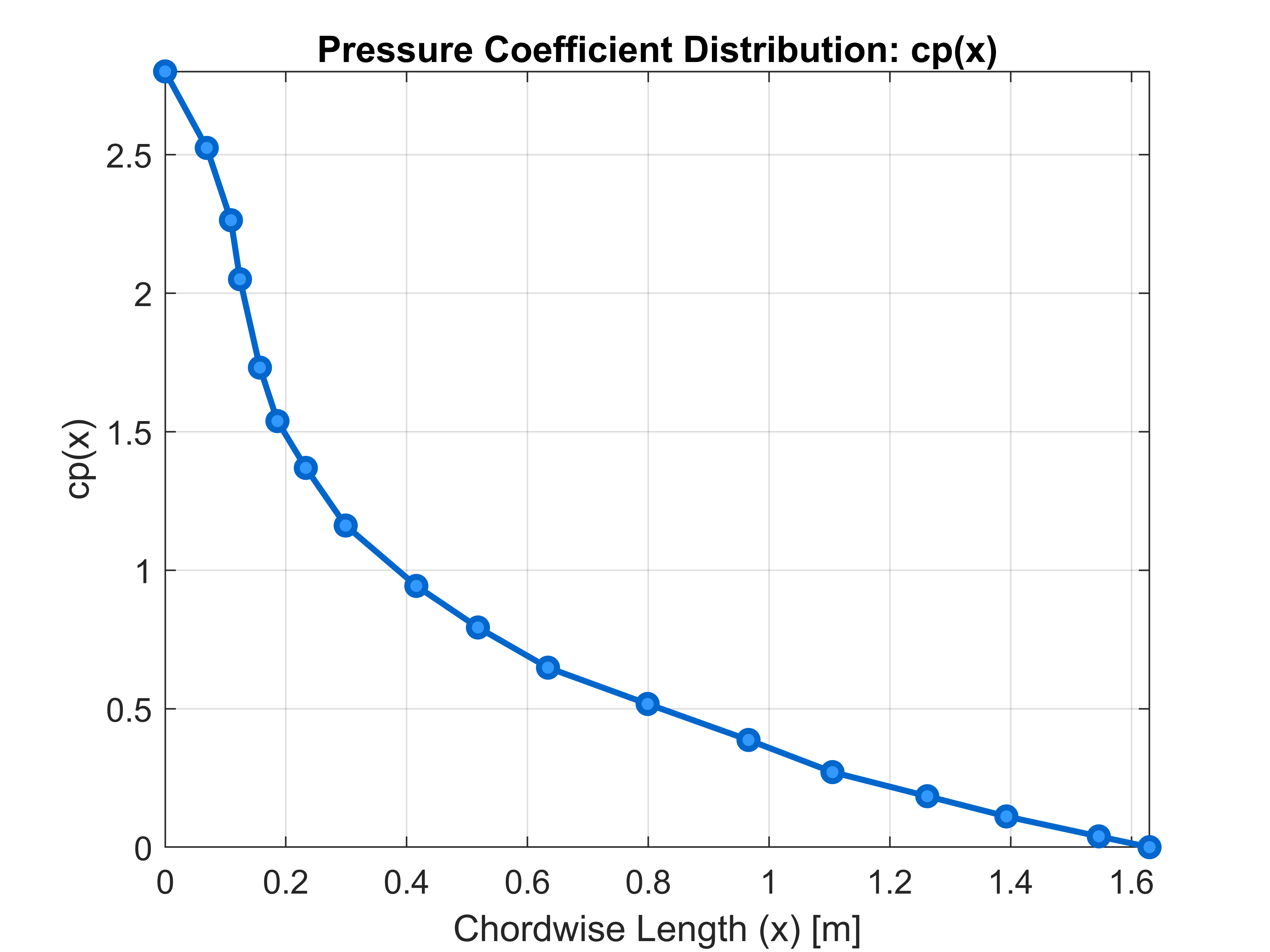
Extrapolated c_p(x)

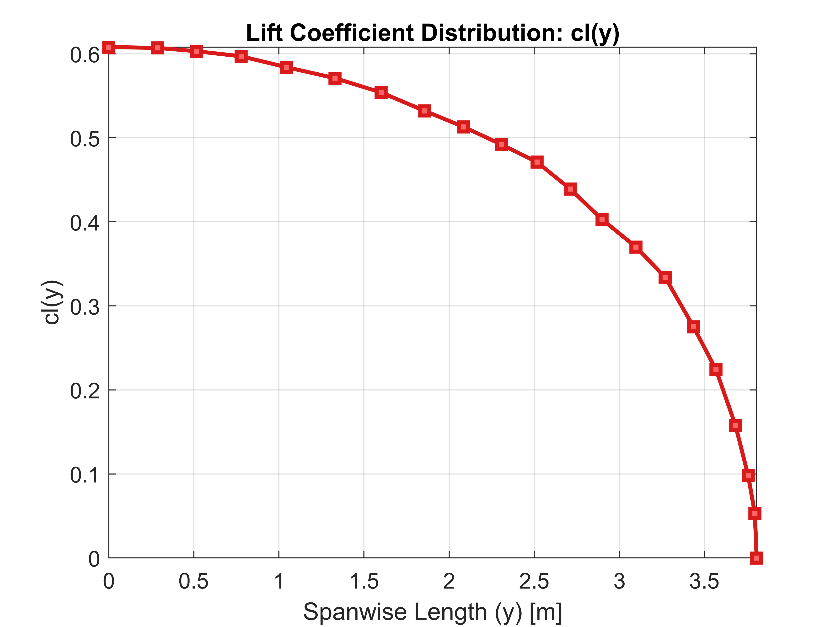
Extrapolated c_l(y)

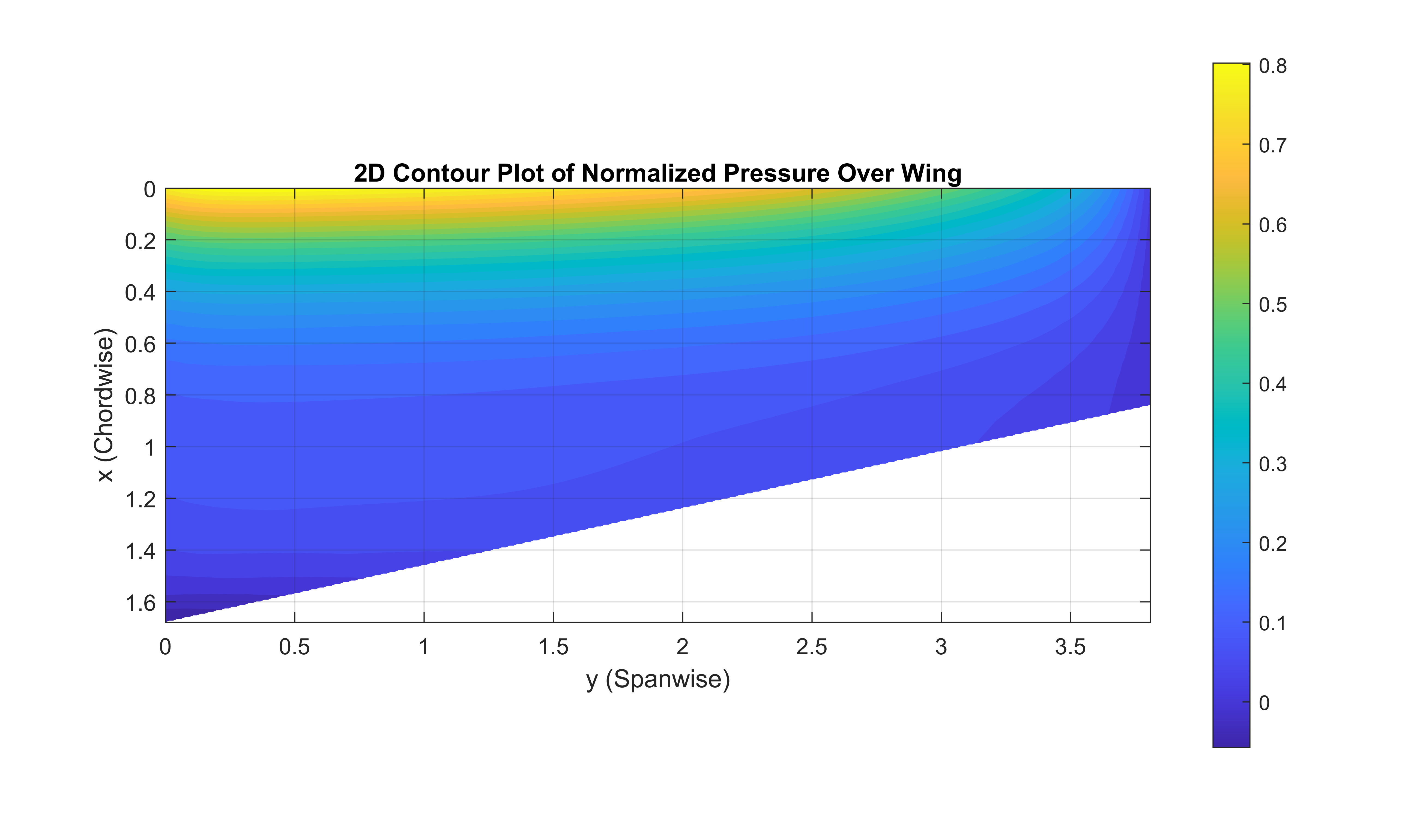
2D Pressure field over the wetted wing surface projection

Control Surface Hingemoment Analysis

For calculating the control surface force, hingemoment approximation found in Roskam Airplane Design Part VI Chapter 10 was used. Specifically, a Three-Dimensional Control Surface and Tab Hingemoment Derivatives method was used. The three-dimensional hingemoment coefficient for a control surface is estimated from:

c_h = c_h0 + c_hα α + c_hδ δ + c_hδt δ_t

ch0 - zero angle of attack, zero control surface deflection and zero tab deflection hingemoment coefficient – for symmetric airfoils equals 0
chα - three dimensional control surface hingemoment derivative due to angle of attack
chδ - three dimensional control surface hingemoment derivative due to control surface deflection
chδt - three dimensional control surface hingemoment derivative due to a tab deflection

Calculating c_hα

First step is to calculate chα and needed variables.

c_hα = [A · cos(Λ_c/4)] / [A + 2 · cos(Λ_c/4)] · (c_hα)_M + Δc_hα

Because there is no sweep angle on the wing, cos(Λc/4) = 0.

(c_hα)_M = (c_hα)_balance / √(1 - M²)

(chα)balance is calculated from all the necessary parameters found in Fig.10.65a.

Since there is no overhang, balance ratio is equal to tc / (2 cf) = 84 / (2 × 260) ≈ 0.162, making
(chα)balance / c"hα ≈ 0.91 (Read from diagram below for round nose).

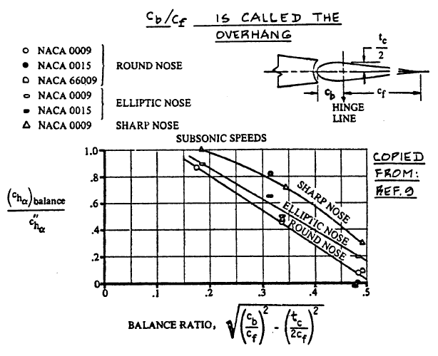
Effect of Nose Shape and Balance on the Two-Dimensional Hingemoment Derivative due to Angle of Attack

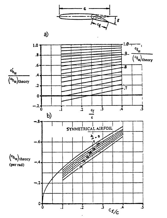
c"hα is obtained from:

c"_hα = c'_hα + 2 (c_lα)_theory [1 - {c_lα / (c_lα)_theory}] {tan(Φ'_te / 2) - (t / c)}

c'_hα = (c'_hα / (c_hα)_theory) (c_hα)_theory

Per the instructions for Eq. 10.128, if the condition:

tan((Φ'_te) / 2) = tan((Φ''_te) / 2) = tan(Φ_te / 2) = t / c

is satisfied, then c''hα = c'hα. This then leads to
c''hα = 0.77 × -0.4 = -0.308. Proof of Eq. 10.128 shows that the upper and lower boundaries of the trailing edge are non-curved lines.

Two-Dimensional Control Surface Hingemoment Derivative due to Angle of Attack

This leads us to finally being able to get (Chα)balanced. If (chα)balanced / c"hα ≈ 0.91 then (chα)balanced = -0.2803.

Now that we know (chα)balanced, we can calculate (Chα)M for M = 0.35 (V_NE≈119 m/s).

(C_hα)_M = -0.2992

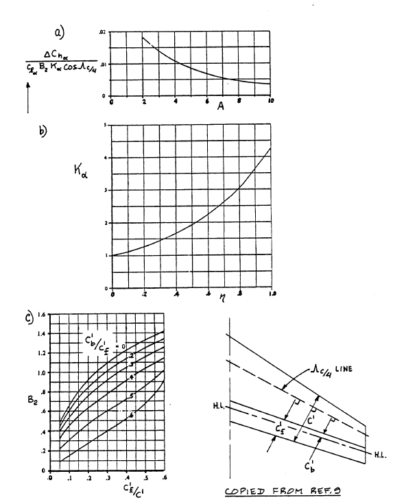
ΔC_hα = ((ΔC_hα) / (c_lα B₂ K_α cosΛ_c/4)) × (c_lα B₂ K_α cosΛ_c/4)

((ΔChα) / (clα B2 Kα cosΛc/4)) - a factor obtained from Figure 10.77a
clα - airfoil lift-curve slope of the surface to which the control surface is attached
B2 – accounts for control surface and balance chord ratios – determined from Figure 10.77c
Kα – accounts for the effect of control surface span – found from:

K_α = [ (K_α)_ηi (1 - η_i) - (K_α)_η0 (1 - η₀) ] / (η₀ - η_i)

ηi – inboard span station of the control surface as a fraction of the main surface semi-span
(Kα)ηi – found from Figure 10.77b
η0 – outboard span station of the control surface as a fraction of the main surface semi-span
(Kα)η0 – found from Figure 10.77b

Reading the diagram in Fig.10.77a, ((ΔChα) / (clα B2 Kα cosΛc/4)) for aspect ratio of 8.23 is 0.004.

Since the aileron spans from 25.2% of the wingspan inboard all the way to the wing tip, η0 will be 1, because the aileron's outward rib is colinear to the wing's tip rib. For ηi = 0.252, (Kα)ηi = 1.35. For η0 = 1, (Kα)η0 = 4.25. Considering this:

K_α = 1.35

B2 is obtained from diagram in Fig.10.77c for c'f / c' ≈ 0.2063.

B₂ = 1.05

Clα was calculated in XFLR5 and is valued at 0.11848.

Three-Dimensional Correction Factors for the Control Surface Hingemoment Derivative due to Angle of Attack

We can now calculate for extrapolated values, ΔChα:

ΔC_hα = 0.0006718

Finally, we can obtain the final value of three dimensional control surface hingemoment derivative due to angle of attack:

C_hα = -0.2986

Calculating C_hδ

Second step is the calculation of Chδ:

C_hδ = (cosΛ_c/4) (cosΛ_hl) × [ (c_hδ)_M + α_δ (c_hα)_M ( (2 cosΛ_c/4) / (A + 2 cosΛ_c/4) ) ] + ΔC_hδ

(chα)M = -0.2992
(chδ)M = (chδ)bal / √(1 - M²)
αδ = 0.5 (obtained from Fig.8.17 for 30° aileron deflection)

We will start with (chδ)M. Solution to this coefficient follows the same path as the one for (Chα)M, so any unnecessary descriptions will be omitted for this step.

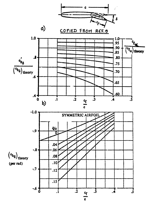
(c_hδ)_bal = c"_hδ × { (c_hδ)_bal / c"_hδ }

c"_hδ = c'_hδ + 2 (c_lδ)_theory × [1 - { c_lδ / (c_lδ)_theory }] × { tan(Φ'_te/2) - (t/c) }

(chδ)bal / c"hδ ≈ 0.91

Because it was proven before that c"hδ = c'hδ, it follows that:

c"_hδ = (c'_hδ / (c_hδ)_theory) × (c_hδ)_theory

c"_hδ = 0.91 × -0.77 = -0.7007

Two-Dimensional Control Surface Hingemoment Derivative due to Control Surface Deflection

For the round nose and a balance ratio of 0.162, reading a diagram in Fig.10.71, we find (chδ)balance to be around -0.5676.

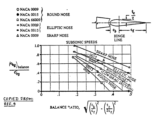
Effect of Nose Shape and Balance on the Two-Dimensional Control Surface Hingemoment Derivative due to Control Surface Deflection

Finally we get:

(c_hδ)_M = (c_hδ)_bal / √(1 - M²) = (-0.5676) / √(1 - 0.35²) = -0.6059

Next, we ought to calculate ΔChδ:

ΔC_hδ = ((ΔC_hδ) / (c_lδ B₂ K_δ cosΛ_c/4 cosΛ_hl)) × (c_lδ B₂ K_δ cosΛ_c/4 cosΛ_hl)

The first member of the equation is a factor obtained from Fig.10.78a.

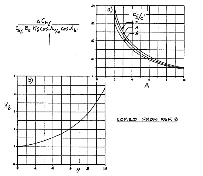
Three-Dimensional Correction Factors for the Control Surface Hingemoment Derivative due to Control Surface Deflections

clδ is found in Fig.8.14 with the value of 0.37. Kδ is basically the same as Kα with a different index and has the same value of 1.35. Same goes for B2, which is 1.05.

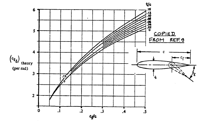
Lift Effectiveness of a Plain Flap

We can now get ΔC_hδ:

ΔC_hδ = 0.009 × 0.37 × 1.05 × 1 = 0.00349

Lastly,

C_hδ = 1 × [ -0.6059 + 0.5 × (-0.2992) × (2 / (8.23 + 2)) ] + 0.00349
C_hδ = -0.6314

Since tab isn't considered in the design, three-dimensional control surface hingemoment derivative due to a tab deflection will be considered zero.

Final Results

After calculating the needed coefficients, we get estimated total three-dimensional hingemoment coefficient for a control surface:

C_h = C_hα α + C_hδ δ = -0.2986 × 0.1658 - 0.7239 × 0.5236
C_h = -0.4285

Negative coefficient value means the moment is acting opposite to the direction of the control surface deflection. Basically, the force acting upon the control surface wants it to return to the neutral position.

If hingemoment equals:

M_hinge = (1/2) ρ_∞ v_∞² S_aileron MAC_aileron C_h
ρ_∞ = 1.225 kg/m³
v_∞ = 119 m/s
S_aileron = 0.9868125 m²
MAC_aileron = 0.34625 m
|M_hinge| = 1269.92 Nm

Force on hinge:

F_hinge = M_hinge / 0.25 MAC_aileron
F_hinge = 109.92 N

Multiplying Fhinge by a loading factor of 12G gives the hinge force applied to the aircraft under maximum loading conditions:

F_hinge12g = 1318.94 N

This force will be applied to the rib edges in the direction of the lift.